Read GIRF tutorial and access related material such as references, scripts and demo data. The demos were presented at the Skope User Meeting 2024, held in Tübingen, September 3.

Vencel Somai, PhD
The gradient system of an MR scanner plays a central role in image formation. Since the 1970s, when the phenomenon that by making the magnetic field deliberately ununiform the MR signal can be spatially encoded was discovered, the gradient technology has improved enormously. Nevertheless, the realms of engineering and MR physics still impart substantial discrepancy between theory and the actual encoding field generated by the MR scanner even nowadays. These encoding errors propagate into the acquired MR signal and ultimately result in image artefact sometimes rendering the collected data unusable. The source of encoding errors is manyfold including bandwidth limitations of gradient amplifiers, eddy currents induced in gradient coils and in other conducting structures of the scanner, field fluctuations caused by mechanical vibrations after gradient switching, and thermal variation in hardware components. These imperfections are often assumed to be linear therefore their superposition can effectively be characterised by a net impulse response function that describes the collective behaviour of the gradient system without having to separate the individual sources. This net impulse response function is usually referred to as Gradient Impulse Response Function (GIRF). Knowing the GIRF enables correcting the acquired MR imaging data for hardware-related encoding imperfections thereby eliminating the associated artefacts and yielding superior image quality. It also enables the more precise design of diffusion, flow, crusher, spoiler etc. gradient lobes for enhanced efficiency and more precise tissue characterisation.
Step 1
The objective of characterisation measurements is to accurately determine the GIRF with sufficient bandwidth and frequency resolution. This is done by observing the response of the gradient system to a test gradient waveform input. The most often employed test waveforms are triangle blips and chirps:
- Short triangle blips are the closest feasible approximation of a Dirac delta function, the theoretically ideal test waveform that evenly covers the whole frequency spectrum. By running an array of experiments where the moment of the triangle blip waveform is varied in incremental steps while keeping the slope constant the response of the gradient system is characterised over the range of frequencies where the GIRF is expected to be non-zero
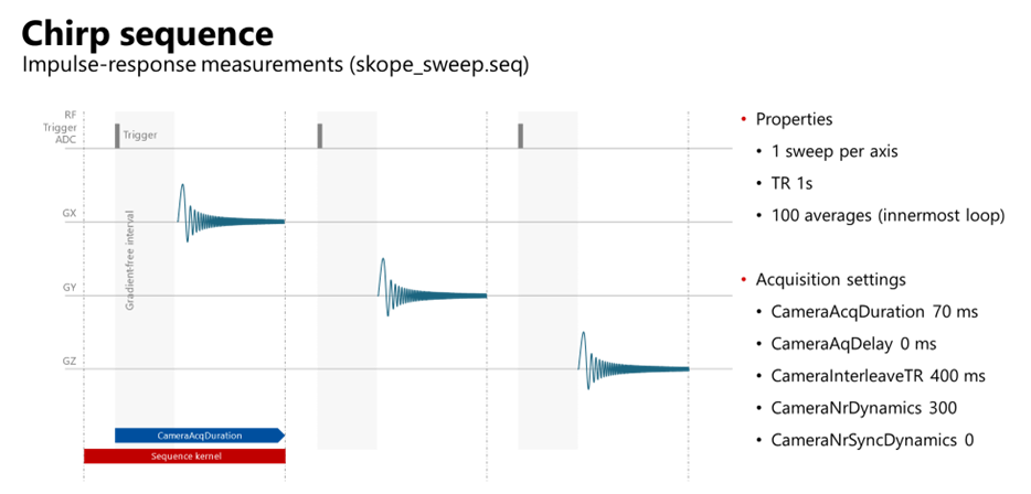
- In case of chirp test waveforms, that also have essentially flat energy distribution in the frequency domain, the sweep speed is varied to probe the entire bandwidth of the GIRF
The output i.e., the response of the gradient system can be measured by a Dynamic Field Camera:

The easiest way to implement a GIRF measurement on your scanner:
- Download the sequences used in the SUM 2024 demo from GitHub:
- git clone https://github.com/SkopeMagneticResonanceTechnologies/Pulseq-Sequences/tree/skope-user-meeting-2024
- Get Pulseq – available on GitHub
- git clone [email protected]:pulseq/pulseq.git
- Interpreter sequences available for Siemens and GE
- Run the Pulseq sequence called skope_gtf.seq and execute a Field Camera measurement using the acquisition parameters given in the figure below.

Additionally or alternatively, sweep gradient pulses can be played out. Run the Pulseq sequence called skope_sweep.seq and execute a Field Camera measurement using the acquisition parameters given in the figure below.

Since the core assumption for the creation of a GIRF is the linearity and time-invariance of the system, it is worthwhile to validate this expectation via a measurement. The linearity check entails playing out two gradient blips with the same length but half the amplitude/slew rate. The system is linear if the measured amplitudes scale correctly:

The steps of performing the linearity check are the same as for the GIRF measurement only the Pulseq file and the acquisition parameters in skope-fx are different:

Step 2
Once sufficient GIRF measurement data has been collected, the GIRF can be estimated using its defining equation:

where o(t) = i(t) is the output field measured by the field camera, i(t) is the nominal input waveform convolved by h(t) i.e., the GIRF. In Fourier domain the convolution is simplified to multiplication therefore it is more practical to derive an estimate for the Fourier-transform of the GIRF, H(ω):

The summation, indexed by j, runs over the measurements corresponding to different input-blips and/or chirps. The workflow of GIRF estimation is summarized in figure below.

The nominal gradient waveform ij(t)=Gj,nom can be obtained by simulating the pulse sequence in the Pulseq sequence simulator. oj(t)=Gj,meas is derived by field monitoring the individual input-blip measurements. More information as well as code to calculate the GIRF are available at: https://github.com/MRI-gradient/girf.
See also the doctoral thesis by Johanna Vannesjö “Characterizing and Correcting for Imperfect Field Dynamics in Magnetic Resonance Imaging”.
Step 3
Knowledge of the GIRF, among other applications, enables k-space trajectory prediction i.e., the prediction of the encoding fields played out by the MR scanner in response to any nominal gradient input. This is important because artefact free image reconstruction requires the precise knowledge of the encoding fields that were present during image acquisition. GIRF-based predictions enable accurate image reconstruction even when direct, concurrent measurement of the encoding fields during image readout is not feasible. Validating the accuracy of a GIRF model and the associated GIRF-based predictions can easily be performed by both predicting as well as concurrently monitoring the encoding fields generated by a given input trajectory.
The examples below illustrate such a comparison for a GRE (on the left) and an EPI (on the right) k-space trajectory. The inset shows zoomed-in views:

The GIRF-predicted k-space trajectory can then be used for more accurate image reconstruction.
Links, scripts, and demo data
- Pulseq
- Skope Pulseq sequences
- GIRF estimation and application code
- Field camera and scanner demo data from Skope User Meeting 2024
- Demo scripts for GIRF prediction and image reconstruction from Skope User Meeting 2024
- For password protected files, please reach out to [email protected] for credentials
- Summary and all other handouts from the Skope User Meeting 2024
